NDIndex Demo - linked-indices

The NDIndex is the simplest index for N-D derived coordinates.

Key concept:

Only manages N-D coordinates (like abs_time with shape (trial, rel_time))
Does NOT manage dimension coordinates - they use default xarray indexing
Enables selection by values in the N-D coordinate

NDIndex is ideal for trial-based neuroscience data, time series with multiple reference frames, or any structured data where you have derived N-D coordinates computed from dimension coordinates.

Note: xarray also has NDPointIndex for spatial nearest-neighbor queries on curvilinear grids. See NDPointIndex vs NDIndex for a comparison of the two approaches.

Diagram showing absolute vs relative time coordinates

from linked_indices import NDIndex
from linked_indices.example_data import trial_based_dataset

Create example data¶

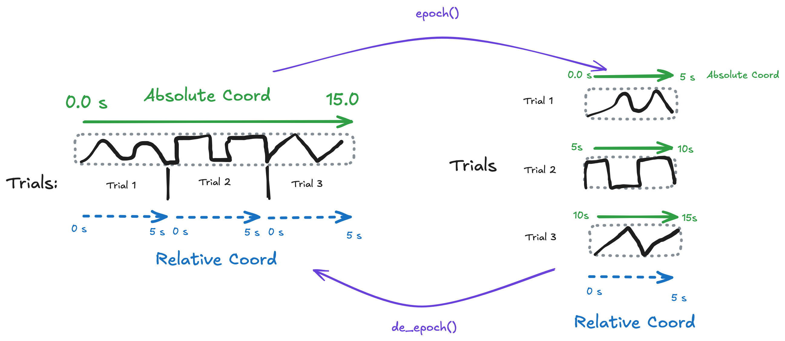
The trial_based_dataset has:

Dimensions: (trial, rel_time)
1D coords: trial, rel_time, trial_onset
2D coord: abs_time = trial_onset + rel_time

ds = trial_based_dataset(mode="stacked")
ds

Apply the NDIndex¶

Only index the 2D abs_time coordinate. The 1D coords keep their default indexes.

ds = ds.set_xindex(["abs_time"], NDIndex)
ds

Selection by abs_time (2D coord)¶

When you select abs_time=7.5:

Default: requires exact match in the N-D array
With method='nearest': finds the cell with value closest to 7.5

The index returns slices for both dimensions that select that cell.

ds.sel(abs_time=7.5)

Range selection on abs_time¶

Slice selection finds all cells where the value falls within the range, then returns the bounding box in each dimension.

ds.sel(abs_time=slice(2.5, 7.5))

⚠️ Slice selection returns bounding boxes¶

Important limitation: When you use sel(coord=slice(start, stop)) on an N-D coordinate, NDIndex returns the bounding box of all matching cells—not just the cells themselves.

                         abs_time values shown in each cell
                         ──────────────────────────────────
                              rel_time: 0    ...    5
                                        ↓           ↓
abs_time array:          ┌─────────────────────────────┐
       trial 0 (cosine)  │ 0.0   0.1   ...   4.9   5.0 │  (abs_time = 0 + rel_time)
       trial 1 (square)  │ 5.0   5.1   ...   9.9  10.0 │  (abs_time = 5 + rel_time)
       trial 2 (sawtooth)│10.0  10.1   ...  14.9  15.0 │  (abs_time = 10 + rel_time)
                         └─────────────────────────────┘

Matching cells             Result (bounding box)
for abs_time 2.5-7.5:      ─────────────────────
                         ┌─────────────────────────────┐
       trial 0 (cosine)  │      ░░░░░░░░░░░░░░░░░░░░░░ │  ← only right half matches
       trial 1 (square)  │ ░░░░░░░░░░░░░                │  ← only left half matches  
       trial 2 (sawtooth)│                              │  ← no match, EXCLUDED
                         └─────────────────────────────┘
                               ↑                   ↑
                         But result includes ALL rel_time (0 to 5)
                         because that's the bounding box!

The slice abs_time=slice(2.5, 7.5) matches:

cosine: rel_time 2.5–5.0 (where abs_time is 2.5–5.0)
square: rel_time 0.0–2.5 (where abs_time is 5.0–7.5)

The bounding box is the union of these ranges:

trial: indices 0–1 (both have matches)
rel_time: indices covering 0.0–5.0 (union of [2.5, 5.0] and [0.0, 2.5])

So the result includes all rel_time values, even though each trial only partially matches!

Why? xarray’s indexing requires rectangular slices. There’s no way to return “cosine for rel_time > 2.5, square for rel_time < 2.5”.

Workaround: Select the bounding box first, then mask:

result = ds.sel(abs_time=slice(2.5, 7.5))
mask = (result.abs_time >= 2.5) & (result.abs_time <= 7.5)
filtered = result.where(mask)

# Demonstrate bounding box behavior
# Create a fresh dataset for clarity
demo_ds = trial_based_dataset(mode="stacked")
demo_ds = demo_ds.set_xindex(["abs_time"], NDIndex)

print("Dataset structure:")
print(f"  Trials: {list(demo_ds.trial.values)}")
print(f"  Trial onsets: {list(demo_ds.trial_onset.values)}")
print("  Each trial spans rel_time 0.0 to 4.99")
print()
print("abs_time ranges per trial:")
for trial in demo_ds.trial.values:
    t = demo_ds.sel(trial=trial)
    print(
        f"  {trial}: abs_time {float(t.abs_time.min()):.1f} to {float(t.abs_time.max()):.1f}"
    )

Dataset structure:
  Trials: [np.str_('cosine'), np.str_('square'), np.str_('sawtooth')]
  Trial onsets: [np.float64(0.0), np.float64(5.0), np.float64(10.0)]
  Each trial spans rel_time 0.0 to 4.99

abs_time ranges per trial:
  cosine: abs_time 0.0 to 5.0
  square: abs_time 5.0 to 10.0
  sawtooth: abs_time 10.0 to 15.0

# Select abs_time from 2.5 to 7.5
# This should match:
#   - cosine trial: rel_time 2.5-4.99 (abs_time 2.5-4.99)
#   - square trial: rel_time 0.0-2.5 (abs_time 5.0-7.5)
#   - sawtooth trial: NO MATCH (abs_time 10.0-14.99)

result = demo_ds.sel(abs_time=slice(2.5, 7.5))

print("Result of sel(abs_time=slice(2.5, 7.5)):")
print(f"  Trials included: {list(result.trial.values)}")
print(
    f"  rel_time range: {float(result.rel_time.min()):.2f} to {float(result.rel_time.max()):.2f}"
)
print(f"  Result shape: {dict(result.sizes)}")
print()
print("But the ACTUAL abs_time values in result span:")
print(f"  min: {float(result.abs_time.min()):.2f}")
print(f"  max: {float(result.abs_time.max()):.2f}")
print()
print("This includes values OUTSIDE our requested range [2.5, 7.5]!")

Result of sel(abs_time=slice(2.5, 7.5)):
  Trials included: [np.str_('cosine'), np.str_('square')]
  rel_time range: 0.00 to 4.99
  Result shape: {'trial': 2, 'rel_time': 500}

But the ACTUAL abs_time values in result span:
  min: 0.00
  max: 9.99

This includes values OUTSIDE our requested range [2.5, 7.5]!

# Show which cells are OUTSIDE the requested range
outside_range = (result.abs_time < 2.5) | (result.abs_time > 7.5)
n_outside = int(outside_range.sum())
n_total = result.abs_time.size

print(
    f"Cells outside requested range [2.5, 7.5]: {n_outside} / {n_total} ({100 * n_outside / n_total:.1f}%)"
)
print()
print("Per trial breakdown:")
for trial in result.trial.values:
    trial_data = result.sel(trial=trial)
    in_range = (trial_data.abs_time >= 2.5) & (trial_data.abs_time <= 7.5)
    print(
        f"  {trial}: {int(in_range.sum())} in range, {int((~in_range).sum())} outside range"
    )

Cells outside requested range [2.5, 7.5]: 499 / 1000 (49.9%)

Per trial breakdown:
  cosine: 250 in range, 250 outside range
  square: 251 in range, 249 outside range

# Workaround: use .where() to mask values outside the range
mask = (result.abs_time >= 2.5) & (result.abs_time <= 7.5)
filtered = result.where(mask)

print("After applying .where() mask:")
print(f"  Shape unchanged: {dict(filtered.sizes)}")
print("  But values outside range are now NaN")
print()
# Show the data values - NaN where outside range
print("Sample of filtered data (showing NaN for out-of-range cells):")
print(filtered.data.values[:, :5])  # First 5 time points

After applying .where() mask:
  Shape unchanged: {'trial': 2, 'rel_time': 500}
  But values outside range are now NaN

Sample of filtered data (showing NaN for out-of-range cells):
[[nan nan nan nan nan]
 [ 1.  1.  1.  1.  1.]]

Slice methods¶

You can configure how NDIndex handles slice selection using the slice_method option:

Method	Description
`"bounding_box"` (default)	Returns the smallest rectangular region containing all matching cells
`"trim_outer"`	Like bounding_box, but more aggressively trims outer dimension indices

# Default: bounding_box
ds.set_xindex(["abs_time"], NDIndex)

# Alternative: trim_outer
ds.set_xindex(["abs_time"], NDIndex, slice_method="trim_outer")

The slice_method is preserved through isel() operations.

Slice with step¶

You can include a step in your slice selection. The step is applied to the innermost dimension (typically rel_time or similar):

# Select every 2nd point in the abs_time range 0-5
ds.sel(abs_time=slice(0, 5, 2))

This first finds the bounding box for abs_time in [0, 5], then applies step=2 to the inner dimension slice.

Example: If the inner dimension normally covers indices 0-50, a step of 2 gives indices 0, 2, 4, ..., 48, 50—roughly half the points.

# Demonstrate slice with step
# Original data has 500 time points
print(f"Original rel_time size: {ds.sizes['rel_time']}")

# Select abs_time 0-3 with step=5 (every 5th point)
result = ds.sel(abs_time=slice(0, 3, 5))
print(f"After slice(0, 3, 5) rel_time size: {result.sizes['rel_time']}")
print(
    f"Rel_time spacing: {result.rel_time.values[1] - result.rel_time.values[0]:.2f}s (5× original)"
)

Original rel_time size: 500
After slice(0, 3, 5) rel_time size: 61
Rel_time spacing: 0.05s (5× original)

Selection by trial (1D coord, default xarray index)¶

The trial coord uses xarray’s default PandasIndex - our NDIndex doesn’t interfere.

ds.sel(trial="square")

Selection by rel_time (1D coord, default xarray index)¶

ds.sel(rel_time=2.5, method="nearest")

isel works correctly¶

Integer selection with scalars properly drops dimensions.

ds.isel(trial=1)

Plotting works correctly¶

The original bug was that plotting drew too many lines. With NDIndex, plotting works as expected.

The plot below shows each trial with two x-axes:

Bottom axis: rel_time (relative time within each trial, always 0-5s)
Top axis: abs_time (absolute time, offset by trial onset)

import matplotlib.pyplot as plt

fig, axes = plt.subplots(3, 1, figsize=(10, 8), sharex=True)

for i, trial in enumerate(ds.trial.values):
    ax = axes[i]
    trial_data = ds.sel(trial=trial)

    # Plot data vs rel_time
    ax.plot(trial_data.rel_time, trial_data.data, color="C0")
    ax.set_ylabel(f"{trial}")
    ax.set_ylim(-1.2, 1.2)

    # Create twin axis for abs_time
    ax2 = ax.twiny()
    ax2.set_xlim(trial_data.abs_time.values.min(), trial_data.abs_time.values.max())

    if i == 0:
        ax2.set_xlabel("abs_time (s)", color="C1")
        ax2.tick_params(axis="x", colors="C1")
    else:
        ax2.tick_params(axis="x", labeltop=False)

axes[-1].set_xlabel("rel_time (s)")
fig.suptitle("Data by Trial (showing both rel_time and abs_time)", y=1.02)
plt.tight_layout()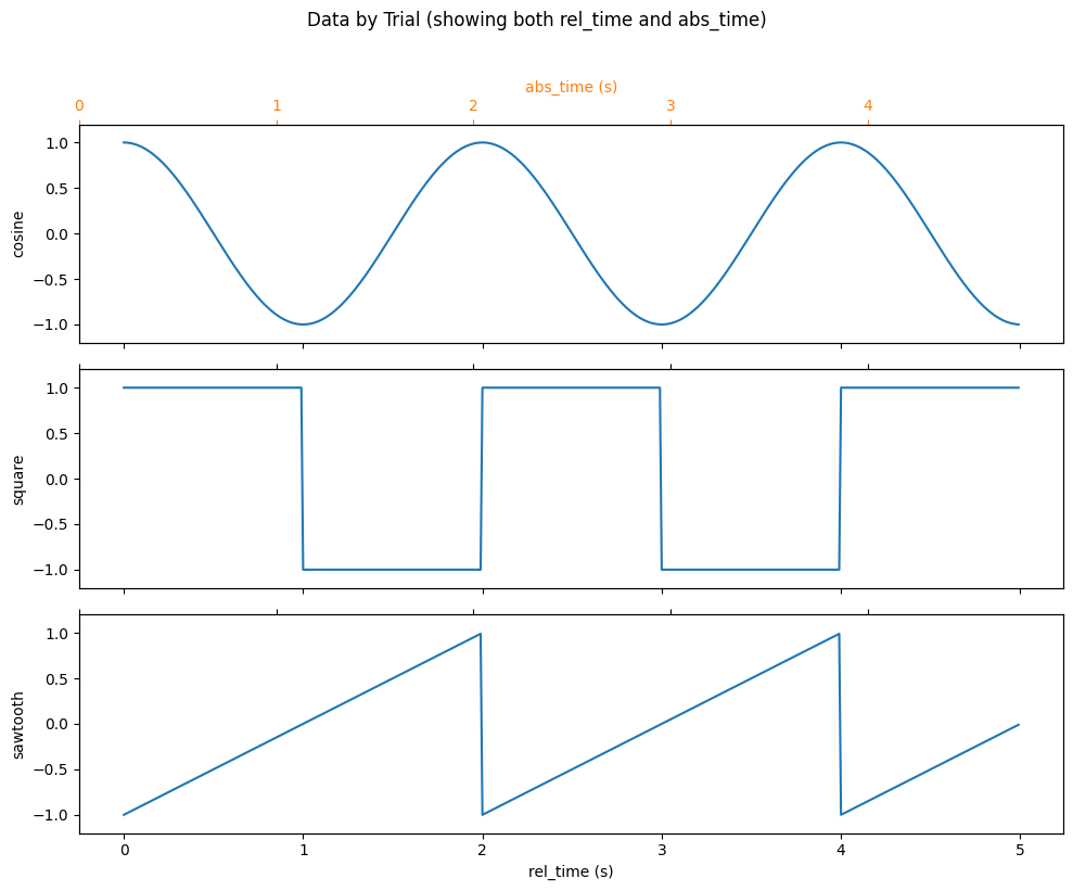

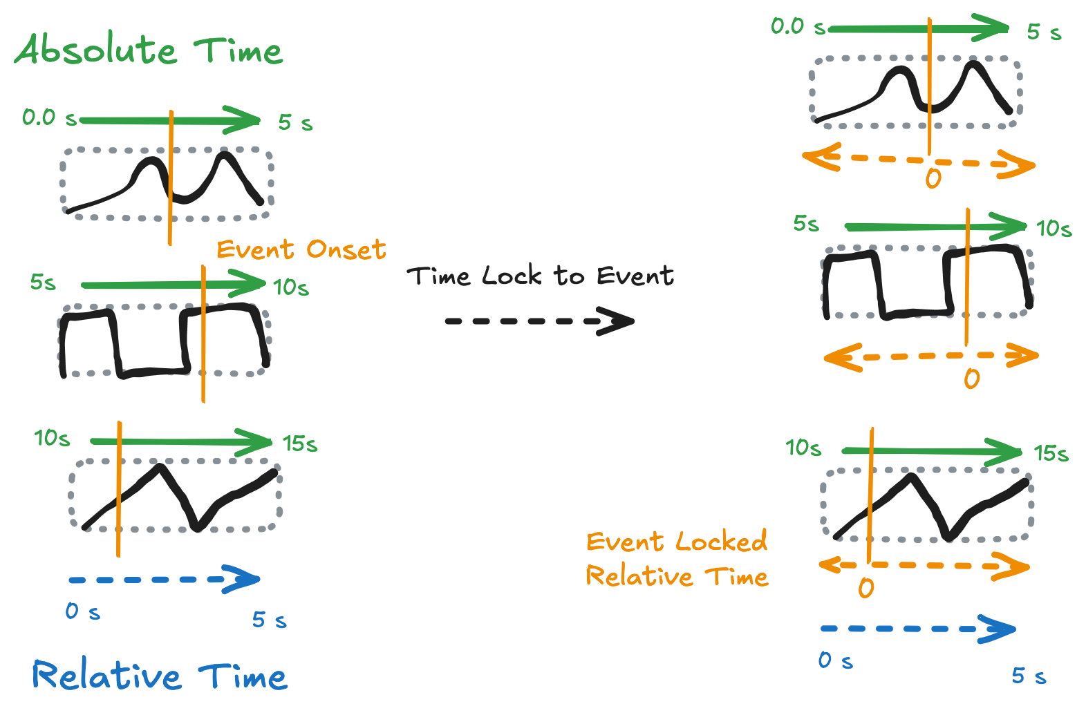
Time-Locking to Events¶

A key use case for NDIndex is time-locking: aligning data to events that occur at different times in each trial. For example, in neuroscience you might want to analyze neural activity relative to:

Stimulus onset (when the stimulus appeared)
Speech onset (when the subject started speaking)
Response time (when they pressed a button)

Each of these events happens at a different time in each trial, creating a 2D time coordinate.

# Add event times that vary per trial
ds = ds.assign_coords(
    {
        "stim_onset": ("trial", [0.5, 0.3, 0.4]),  # When stimulus appeared
        "speech_onset": ("trial", [1.5, 2.5, 3.0]),  # When subject started speaking
        "response_time": ("trial", [2.0, 1.8, 2.2]),  # When they pressed button
    }
)

# Create time-locked coordinates (2D: trial × rel_time)
# These measure time relative to each event
ds = ds.assign_coords(
    {
        "stim_locked": ds["rel_time"] - ds["stim_onset"],
        "speech_locked": ds["rel_time"] - ds["speech_onset"],
        "response_locked": ds["rel_time"] - ds["response_time"],
    }
)

# Add the time-locked coords to the NDIndex for selection
ds = ds.drop_indexes("abs_time").set_xindex(
    ["abs_time", "stim_locked", "speech_locked", "response_locked"], NDIndex
)
ds

# Plot aligned to speech onset - time=0 is when subject started speaking
ds["data"].plot.line(x="speech_locked", row="trial");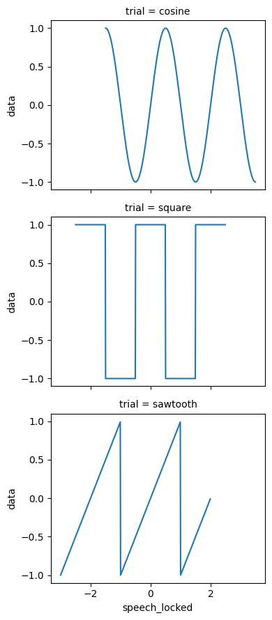

Select by time-locked coordinate¶

Now we can select data relative to events. For example, get the data point closest to 0.5 seconds after speech onset:

# Select 0.5 seconds after speech onset (in each trial)
ds.sel(speech_locked=0.5, method="nearest")

Select a time window around an event¶

Get data from 0.5 seconds before to 1.0 seconds after stimulus onset:

# Select -0.5 to +1.0 seconds around stimulus onset
window = ds.sel(stim_locked=slice(-0.5, 1.0))
window["data"].plot.line(x="stim_locked", row="trial");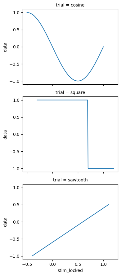

Compare different alignments¶

The same data looks different when aligned to different events. Here we compare stimulus-locked vs response-locked views:

import matplotlib.pyplot as plt

fig, axes = plt.subplots(1, 2, figsize=(12, 4))

# Left: stimulus-locked
for i, trial in enumerate(ds.trial.values):
    trial_data = ds.sel(trial=trial)
    axes[0].plot(trial_data.stim_locked, trial_data.data, label=trial)
axes[0].axvline(0, color="k", linestyle="--", alpha=0.5)
axes[0].set_xlabel("Time from stimulus (s)")
axes[0].set_title("Stimulus-locked")
axes[0].legend()

# Right: response-locked
for i, trial in enumerate(ds.trial.values):
    trial_data = ds.sel(trial=trial)
    axes[1].plot(trial_data.response_locked, trial_data.data, label=trial)
axes[1].axvline(0, color="k", linestyle="--", alpha=0.5)
axes[1].set_xlabel("Time from response (s)")
axes[1].set_title("Response-locked")
axes[1].legend()

plt.tight_layout();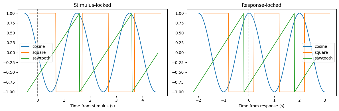

3D Coordinates: Multi-Subject Data¶

NDIndex works with coordinates of any dimensionality ≥2. Here’s an example with 3D absolute time across subjects, trials, and time points.

In multi-subject studies, each subject’s session starts at a different real-world time. The 3D abs_time coordinate captures this:

import numpy as np
import xarray as xr

# Create 3D dataset: 2 subjects × 3 trials × 50 time points
n_subjects, n_trials, n_times = 2, 3, 50

subjects = ["alice", "bob"]
trials = ["trial_0", "trial_1", "trial_2"]
rel_time = np.linspace(0, 1, n_times)

# Each subject's session started at a different time (e.g., different days)
subject_offset = xr.DataArray(
    [0.0, 1000.0], dims=["subject"], coords={"subject": subjects}
)

# Trial onsets within each session
trial_onset = xr.DataArray([0.0, 2.0, 4.0], dims=["trial"], coords={"trial": trials})

# 3D absolute time = subject_offset + trial_onset + rel_time
# Shape: (subject, trial, rel_time) = (2, 3, 50)
abs_time_3d = subject_offset + trial_onset + xr.DataArray(rel_time, dims=["rel_time"])

# Create dataset with random signal data
ds_3d = xr.Dataset(
    {
        "signal": (
            ("subject", "trial", "rel_time"),
            np.random.randn(n_subjects, n_trials, n_times),
        )
    },
    coords={
        "subject": subjects,
        "trial": trials,
        "rel_time": rel_time,
        "abs_time": abs_time_3d,
    },
)

# Apply NDIndex to the 3D coordinate
ds_3d = ds_3d.set_xindex(["abs_time"], NDIndex)
ds_3d

The abs_time coordinate now has shape (subject, trial, rel_time):

Alice's session (offset=0):        Bob's session (offset=1000):
Trial 0: 0.0 → 1.0                 Trial 0: 1000.0 → 1001.0
Trial 1: 2.0 → 3.0                 Trial 1: 1002.0 → 1003.0  
Trial 2: 4.0 → 5.0                 Trial 2: 1004.0 → 1005.0

Selection on 3D coordinates¶

# Find the cell where abs_time ≈ 1002.5 (Bob's session, trial 1, middle)
result = ds_3d.sel(abs_time=1002.5, method="nearest")
print(f"Subject: {result.subject.item()}")
print(f"Trial: {result.trial.item()}")
print(f"Rel_time: {result.rel_time.item():.2f}")
print(f"Abs_time: {result.abs_time.item():.2f}")
result

Subject: bob
Trial: trial_1
Rel_time: 0.49
Abs_time: 1002.49

Dimension reduction with 3D coords¶

When you use isel() with scalar indexers, dimensions are dropped and the N-D coordinate reduces accordingly:

# Select one subject: 3D → 2D (NDIndex stays active)
alice = ds_3d.isel(subject=0)
print(f"After isel(subject=0): abs_time.dims = {alice.abs_time.dims}")
print(f"NDIndex still active: {'abs_time' in alice.xindexes}")

# Select one subject AND one trial: 3D → 1D (NDIndex dropped)
single_trial = ds_3d.isel(subject=0, trial=1)
print(f"\nAfter isel(subject=0, trial=1): abs_time.dims = {single_trial.abs_time.dims}")
print(f"NDIndex dropped (1D coord): {'abs_time' not in single_trial.xindexes}")

After isel(subject=0): abs_time.dims = ('trial', 'rel_time')
NDIndex still active: True

After isel(subject=0, trial=1): abs_time.dims = ('rel_time',)
NDIndex dropped (1D coord): True

Summary¶

The NDIndex enables powerful operations on N-D derived coordinates:

Basic features:

Manages N-D coordinates (2D, 3D, or higher)
Enables sel() on those coordinates to find matching indices
Lets 1D dimension coordinates use default xarray indexing
Properly handles isel() with dimension dropping
Works correctly with plotting

Slice selection options:

slice_method="bounding_box" (default): smallest rectangle containing all matches
slice_method="trim_outer": like bounding_box but trims outer dimensions more aggressively
Step support: sel(coord=slice(start, stop, step)) applies step to innermost dimension

Time-locking workflow:

Add event times as 1D coordinates (per trial)
Create time-locked coordinates: rel_time - event_onset
Add them to NDIndex: set_xindex([...], NDIndex)
Select and plot relative to any event

Limitations:

Slice selection returns bounding boxes, not exact matches
Use .where() for precise filtering after slice selection

This makes it easy to analyze the same data from multiple temporal perspectives—a common need in neuroscience, psychophysics, and other time-series domains.