Hierarchical Cell Data with Relative and Absolute Time

This notebook demonstrates how to use DimensionInterval to model hierarchical experimental data where:

Cells are recorded sequentially, each with their own time window
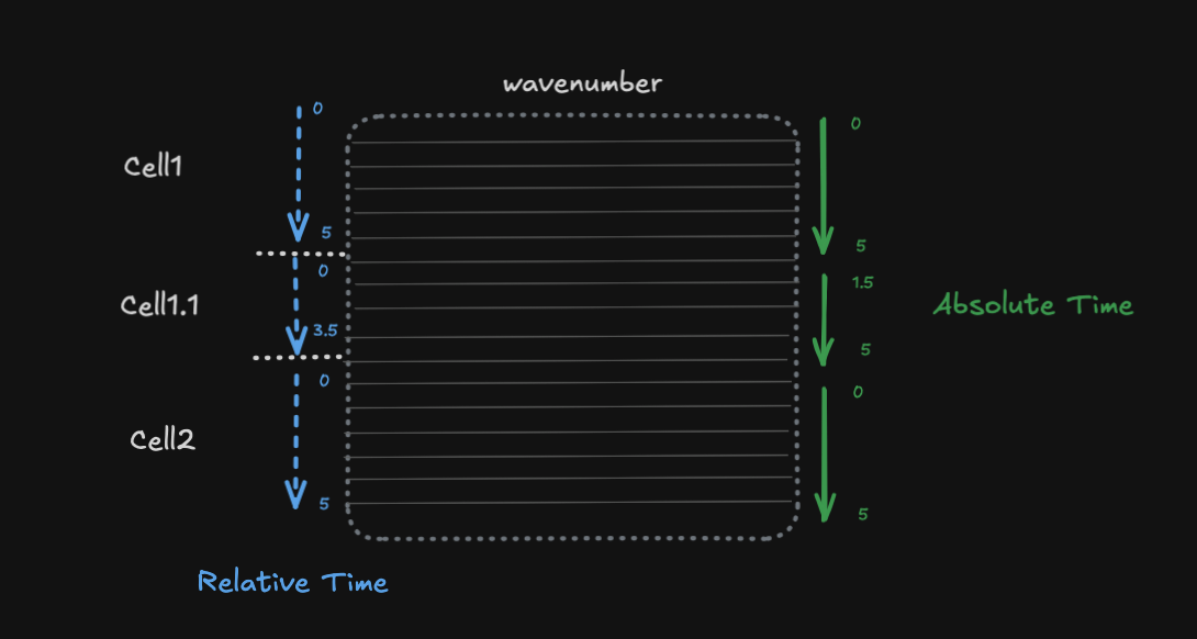
Relative time starts at 0 for each cell (local to the cell)
Absolute time is the global experimental time
Each cell has associated spectral data (e.g., wavenumber measurements)

This is common in experiments where you record from multiple cells/trials sequentially, and want to align data both within-cell (relative) and across the experiment (absolute).

import numpy as np
import xarray as xr
from linked_indices import DimensionInterval

Creating the cell hierarchy¶

We have three cells recorded at different absolute times:

Cell	Absolute Time	Relative Time	Duration
Cell1	0 - 5	0 - 5	5s
Cell1.1	5 - 10	0 - 5 (reset)	5s (3.5s active)
Cell2	10 - 15	0 - 5 (reset)	5s

# Cell definitions with absolute timing
cells = ["Cell1", "Cell1.1", "Cell2"]
cell_abs_onset = np.array([0.0, 5.0, 10.0])  # Absolute start time
cell_duration = np.array([5.0, 5.0, 5.0])  # Duration of each cell recording

# Spectral dimension (wavenumber) - typical spontaneous Raman range
wavenumbers = np.linspace(400, 3400, 1340)  # 400-3400 cm⁻¹, 1340 points

Building the absolute time axis¶

The absolute time runs continuously across the entire experiment (0 to 15 seconds):

# Absolute time axis - continuous across all cells
dt = 0.1  # 100ms resolution
abs_time = np.arange(0, 15, dt)  # 0 to 15 seconds

# Generate synthetic spectral data (wavenumber x absolute_time)
np.random.seed(42)
spectral_data = np.random.randn(len(wavenumbers), len(abs_time))

# Add some structure - different cells have different spectral signatures
for i, (onset, dur) in enumerate(zip(cell_abs_onset, cell_duration)):
    mask = (abs_time >= onset) & (abs_time < onset + dur)
    spectral_data[:, mask] += (i + 1) * 0.5  # Different baseline per cell

Creating the Dataset with DimensionInterval¶

We create a dataset where:

abs_time is the continuous time dimension
cell dimension is linked to abs_time via onset/duration intervals
wavenumber is an independent spectral dimension

# Create the dataset
ds = xr.Dataset(
    {"spectra": (("wavenumber", "abs_time"), spectral_data)},
    coords={
        # Continuous absolute time
        "abs_time": abs_time,
        # Spectral dimension
        "wavenumber": wavenumbers,
        # Cell dimension with onset/duration
        "cell": ("cell", cells),
        "cell_onset": ("cell", cell_abs_onset),
        "cell_duration": ("cell", cell_duration),
    },
)
ds

# Apply DimensionInterval to link abs_time and cell dimensions
ds = ds.drop_indexes(["abs_time", "cell"]).set_xindex(
    ["abs_time", "cell_onset", "cell_duration", "cell"],
    DimensionInterval,
    onset_duration_coords={"cell": ("cell_onset", "cell_duration")},
)
ds

Selecting by cell¶

When we select a cell, the absolute time is automatically constrained to that cell’s interval:

# Select Cell1 - abs_time is constrained to [0, 5)
ds.sel(cell="Cell1")

# Select Cell1.1 - abs_time is constrained to [5, 10)
ds.sel(cell="Cell1.1")

Selecting by absolute time¶

Selecting a time range automatically constrains which cells are included:

# Select time range that spans Cell1 and Cell1.1
ds.sel(abs_time=slice(3, 7))

Adding relative time¶

For within-cell analysis, we often want relative time that starts at 0 for each cell. We can compute this as a derived coordinate:

def add_relative_time(ds_cell):
    """Add relative time coordinate (time since cell onset)."""
    # Get the cell's onset time
    onset = ds_cell.cell_onset.values.item()
    # Compute relative time
    rel_time = ds_cell.abs_time.values - onset
    return ds_cell.assign_coords(rel_time=("abs_time", rel_time))


# Example: Cell1 with relative time
cell1 = add_relative_time(ds.sel(cell="Cell1"))
cell1

# Cell1.1 with relative time - starts at 0 even though abs_time starts at 5
cell1_1 = add_relative_time(ds.sel(cell="Cell1.1"))
cell1_1.rel_time.values[:10]  # First 10 relative time points

Stacking cells with relative time¶

A common analysis pattern is to align all cells by their relative time for comparison. Since each cell has the same duration, we can create a stacked view:

# Create a common relative time axis for stacking
rel_time_common = np.arange(0, 5, dt)


def extract_cell_data(ds, cell_name, rel_time_axis):
    """Extract a single cell's data aligned to a common relative time axis."""
    cell_data = ds.sel(cell=cell_name)
    onset = cell_data.cell_onset.values.item()

    # Get absolute times that correspond to the relative time axis
    abs_times_needed = rel_time_axis + onset

    # Select data at these times (using nearest neighbor for any boundary issues)
    selected = cell_data.sel(abs_time=abs_times_needed, method="nearest")

    return xr.Dataset(
        {"spectra": (("wavenumber", "rel_time"), selected.spectra.values)},
        coords={
            "wavenumber": selected.wavenumber.values,
            "rel_time": rel_time_axis,
        },
    )


# Extract each cell with common relative time axis
cell_datasets = [extract_cell_data(ds, cell, rel_time_common) for cell in cells]

# Stack along cell dimension
stacked = xr.concat(cell_datasets, dim=xr.Variable("cell", cells))
stacked

Now we can easily compare cells at the same relative time point:

# Compare all cells at relative time = 2.5 seconds
stacked.sel(rel_time=2.5, method="nearest")

# Average spectrum across all cells at each relative time point
stacked.spectra.mean(dim="cell")

Summary¶

This example demonstrated:

Hierarchical cell structure - Cells recorded at different absolute times
DimensionInterval linking - Absolute time automatically constrained when selecting cells
Relative time computation - Converting from absolute to within-cell relative time
Stacked analysis - Aligning cells by relative time for cross-cell comparison

The key insight is that DimensionInterval handles the absolute time ↔ cell relationship, while relative time can be computed on-the-fly or stored as an additional coordinate for within-cell analysis.